Visualising language similarities without trees

Gerhard Jäger uses lexostatistics to demonstrate that language similarities can be computed without using tree-based representations (for why this might be important, see Kevin’s post on reconstructing linguistic phylogenies).  On the way, he automatically derives a tree of phoneme similarity directly from word lists.  The result is an alternative and intuitive look at how languages are related (see graphs below).  I review the method, then suggest one way it could get away from prior categorisations entirely.

Jäger presented work at the workshop on Visualization of Linguistic Patterns and Uncovering Language History from Multilingual Resources at the recent EACL conference last month.  He uses the Automated Similarity Judgment Program (ASJP) database, which contains 40 words from the Swadesh-list (universal concepts) for around 5800 languages (including Klingon!).  The words are transcribed in the same coarse transcription.  The task is to calculate the distance between languages based on these lists in a way that they reflect the genetic relationships between languages.

The LDND distance measure is used as a starting point (Bakker et al. 2009):  Given two languages, the distance between them is the average normalised Levenshtein distance between each word pair.  That is, the average proportion of phonemes that need to be changed in order to transform a word in one language to a word in the other.   The measure is further normalised by the average distance between all non-synonymous words from the two languages.  This controls for the fact that if the two languages have large phoneme inventories with little overlap, the distance measure will be disproportionately high.

Weighting phoneme changes

Jäger improves this measure in two ways.  First, the distance measure is unrealistic because it treats the distance between all phonemes as the same.  Intuitively, the change between [hand] and [hent] is closer than [hand] and [mano], even though both paris differ in two phonemes.  What is needed is a way to weight each phoneme change by its linguistic plausibility.  For example, an [i] is more likely to change diachronically to a [j] than to a [k].

Luckily, there is a similar problem in bioinformatics when trying to align genetic protein sequences.  The best alignment is the one that has the most evolutionarily plausible mutations.  Phonetic representations of words can be aligned in the same way.  For instance, the Spanish and German word for ‘star’ (estrella and Stern) can be aligned as follows:

Spanish est-reya
         || ||
German  -StErn--

While this aligns two implausible changes (e and n), it also aligns a plausible one (s and S, alveolar and postalveolar fricatives).  The algorithm to discover the weights assumes that more plausible alignments will occur within related languages.  The weighting is calculated according to the following formula (based on the formula for the The Block Substitution Matrix):

where p[ij] is the probability of amino acid i aligning with amino acid j and q[i] is the frequency of i.

For phonemes, the frequencies can be calculated from the frequencies of phonemes in the ASJP database.  Jäger calculates p using the following algorithm:

1. Pick two languages from the same language family at random
2. Pick a meaning
3. Align the two words from each langauge that correspond to this meaning using a distance metric.
4. For each aligned phoneme pair, add one to that pair’s frequency

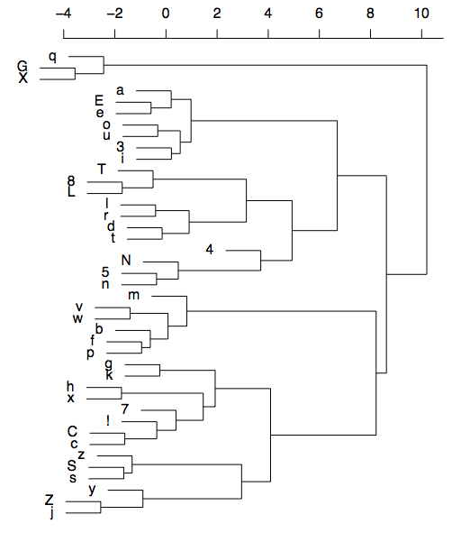
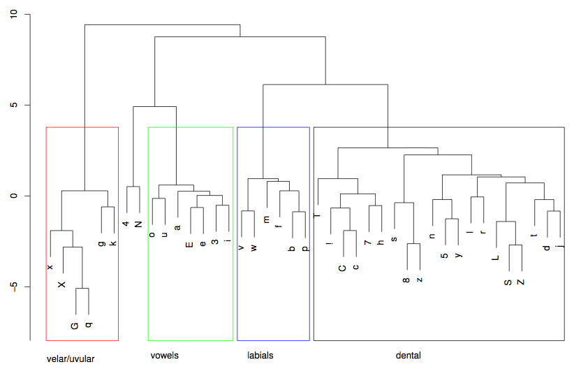
The distance metric could be the Levenshtein distance, the LDND distance or the Needleman-Wunsch algorithm (used in alignment of protein sequences).  This algorithm is repeated 100,000 times.  Because the algorithm compares synonymous words in related languages, it is more likely to sample phoneme pairs that are related by descent, and therefore similar.  This results in the following classification (from Jäger, 2012, p.4, visualised using hierarchical clustering):

 

The results are phonetically plausible – the vowels are together and there are sensible clusterings such as S and tS, and the nasal cluster (N, 5 n) and so on.  The frequencies can be translated into weights for use in the distance measures.

Further improvements

The second improvement on the LDND measure is to take account of the variance in as well as the average of the distance between all non-synonymous word pairs. Jäger uses an information-theoretic approach to incorporate the variance.  Essentially, this is the amount of information that you gain about a word by knowing its translation in another language (see page 4).

Jäger then compares the different similarity measurements under this approach.  Jäger’s algorithm using the Needleman-Wunsch distance metric performed better than when using the Levenshtein distance metric or the original LDND algorithm (although the effect size is small).

Visualising the differences between languages

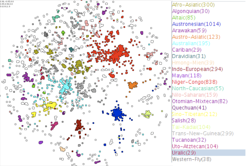
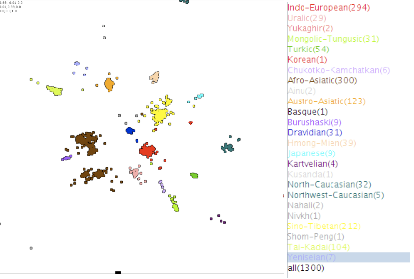
Finally, the distances between languages were visualised using a force directed graph layout (using the free CLANS software).  Basically, each language is represented by a particle in space that is attracted to similar languages and repelled by dissimilar languages.  The CLANS program simulates the particles moving until they reach an equilibrium.

Below is the result for all languages:

And for Eurasian languages:

Jäger describes the data for Eurasian languages as following:

“The Dravidian languages (dark blue) are located at the center. AfroAsiatic (brown), Uralic (pink), Indo European (red), SinoTibetan (yellow), Hmong Mien (light orange), AustroAsiatic (orange), and TaiKadai (yellowish light green) are arranged around the center. Japanese (light blue) is located further to the periphery outside SinoTibetan. Outside IndoEuropean the families Chukotko Kamchatkan (light purple), MongolicTungusic (lighter green), Turkic (darker green) Kartvelian (dark purple) and Yukaghir (pinkish) are further towards the periphery beyond the Turkic languages. The Caucasian languages (both the North Caucasian languages such as Lezgic and the Northwest Caucasian languages such as Abkhaz) are located at the periphery somewhere between IndoEuropean and SinoTibetan. Burushaski (purple) is located near to the Afro Asiatic languages. Some of these pattern coincide with proposals about macrofamilies that have been made in the literature. For instance the relative proximity of IndoEuropean, Uralic, ChukotkoKamchatkan, MongolicTungusic, the Turkic languages, and Kartvelian is reminiscent of the hypothetical Nostratic superfamily. Other patterns, such as the consistent proximity of Japanese to Sino Tibetan, is at odds with the findings of historical linguistics and might be due to language contact. Other patterns, such as the affinity of Burushaski to the AfroAsiatic languages, appear entirely puzzling.”

The result is impressive, given that it’s a clustering of languages calculated directly from words which can be run on an ordinary laptop in a few hours.  It’s easy to imagine extensions to this by adding more cultural variables or socio-economic data.  It would be interesting to see how well the visualisation corresponded to a physical map of the world, perhaps by simulating the particles in an additional field with repelling areas representing the oceans.

Removing trees altogether

Jäger notes that the advantage of the CLANS approach is that, unlike SplitsTree or phylogenetic techniques, it does not use or estimate an underlying tree structure.  Patterns that were previously hidden may be discovered by this kind of visualisation.  However, this claim is somewhat undermined by the approach taken:  The algorithm for calculating the phoneme alignment weightings uses data about language families – which is itself part of a tree-like classification.  Without this information, the algorithm would pick unrelated words more frequently and the measure would be less accurate.  it seems that getting away from trees is difficult (see also Kevin’s post on reconstructing phylogenies)

I propose an alternative to Jäger’s algorithm which does not rely on any language classifications.  Instead of picking language pairs by family, we can pick them by physical proximity.  The languages in the ASJP database have information from the Ethnologue, including geographic co-ordinates of the center of the language community.  The alternative algorithm is thus:

1. Pick a language pair with a probability inversely proportionate to the physical distance between them.
2. Pick a meaning
3. Align the two words from each langauge that correspond to this meaning using a distance metric.
4. For each aligned phoneme pair, add one to that pair’s frequency

I actually used the cubed inverse of the great arc distance in kilometers.  It’s not clear whether this metric would work.  Clearly, languages that are physically close should have a shared history, but the measure does not take into account physical barriers like oceans or flat, open ground compared to mountainous terrain.  I tested this algorithm on Indo-European languages for 200,000 runs.  Below are the results, displayed in the same format as Jäger (2012) on the left and the same tree with IPA symbols on the right (click for larger image).

Although the results are somewhat different to that in Jäger (2012), they are also phonetically plausible.  The vowels are together, there are clusters of dental, alveolar and bilabial phonemes and there are affricate-fricative pairs.  It seems realistic, then, that this visualisation approach could work entirely without prior data on language classifications.  I tried running it on the data for all languages, but with 6 million language pairs, my poor python script was too slow!  Let me know if you’d like to see the code.

———

UPDATE:

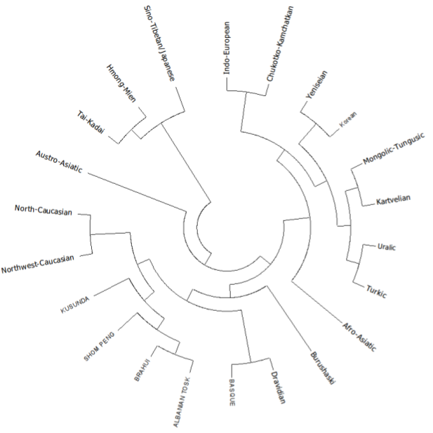
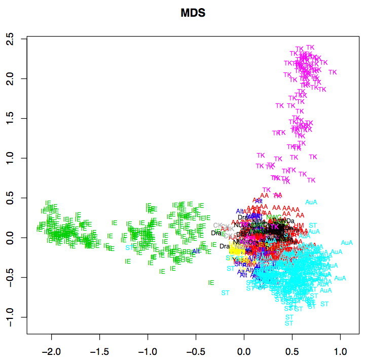
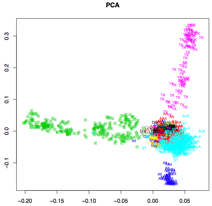
First, between writing the paper and giving the talk, Jäger improved the method and compared this visualisation to some other methods such as Neighbour-Joining tree, multidimensional scaling and Principal  components analysis.  Some informative slides can be found here.

Below are some of the alternative visualisations (click for larger image).  Jäger points out that PCA is only really useful for the large language families, while CLANS is sensitive to local patterns.

The phoneme diagram is also updated in the talk slides, and actually resembles mine more (I assume Jäger means ‘Coronal/Dorsal’ instead of ‘dental’ below):

 

Also, Jäger took the phoneme distance measures produced by my variation of the algorithm above and computed the similarity matrix for Indo-European languages.  The Neighbor Joining tree computed from this has 51 false positives (17%), while the original algorithm produces 87 false positives.  So, far from being a coarse approximation, the distance measure has actually improved the performance!  The comparison is not entirely fair, however, since I ran my algorithm for twice as long as Jäger.  Still, this is an interesting development.

 

References

Jäger, G. (2012) Estimating and visualizing language similarities using weighted alignment and force-directed graph layout, to appear in Proceedings of LINGVIS & UNCLH, Workshop at EACL 2012, Avignon.

Wichmann, Søren, André Müller, Viveka Velupillai, Annkathrin Wett, Cecil H. Brown, Zarina Molochieva, Julia Bishoffberger, Eric W. Holman, Sebastian Sauppe, Pamela Brown, Dik Bakker, Johann-Mattis List, Dmitry Egorov, Oleg Belyaev, Matthias Urban, Harald Hammarström, Agustina Carrizo, Robert Mailhammer, Helen Geyer, David Beck, Evgenia Korovina, Pattie Epps, Pilar Valenzuela, and Anthony Grant. (2012). The ASJP Database (version 15).

Frickey T., Lupas A.N. (2004) CLANS: a Java application for visualizing protein families based on pairwise similarity. Bioinformatics 20:3702-3704

Bakker, D., Müller, A., Velupillai, V., Wichmann, S., Brown, C., Brown, P., Egorov, D., Mailhammer, R., Grant, A., & Holman, E. (2009). Adding typology to lexicostatistics: A combined approach to language classification Linguistic Typology, 13 (1), 169-181 DOI: 10.1515/LITY.2009.009