More on Phoneme Inventory Size and Demography

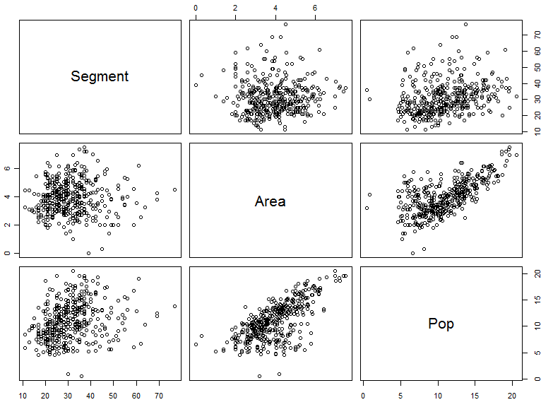
On the basis of Sean’s comment, about using a regression to look at how phoneme inventory size improved as geographic spread was incorporated along with population size, I decided to look at the stats a bit more closely (original post is here). It’s fairly easy to perform multiple regression in R, which, in the case of my data, resulted in highly significant results (p<0.001) for the intercept, area and population (residual standard error = 9.633 on 393 degrees of freedom; adjusted R-Squared = 0.1084). I then plotted all the combinations as scatterplots for each pair of variables. As you can see below, this is fairly useful as a quick summary but it is also messy and confusing. Another problem is that the pairs plot is on the original data and not the linear model.

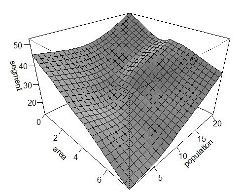
We can go further and use a non-parametric local regression model (Fox, 2005). The problem here, however, is there are no parameter estimates, so to see the result of the regression we have to view the fitted regression surface graphically:

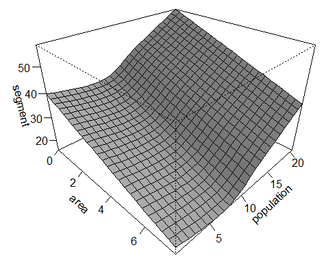
Make what you will of the plotted regression surface — for me it seems largely in agreement with the correlation I performed in the previous post. We can address the statistical significance of each predictor (area and population) by dropping it from the model and performing an approximate incremental F-test for the change in the residual sum of squares. Again, this returns highly significant results for both area (F-value = 40290; p<0.001) and population (F-value = 34364; p<0.001). With the relationship of segment inventory to area and population appearing to be non-linear we can also use a Generalised Additive Model (GAM). This model allows you specify a distribution (in this case a Gaussian), which can then be viewed with a fitted surface for the additive non-parametric regression of segment inventory on area and population (see bottom left).

The general dynamic is now slightly clearer: a decreasing area and increasing population tends to correlate with a larger phoneme segment inventory. Exactly what I’d expect on the basis of my social interconnectedness scale — a large population spread over a small geographic area. Again, the model returns highly significant results for the intercept, area and population (p<0.001; R-Squared (adjusted): 0.132; Deviance explained: 14.2%). I’m cautious of reading too much into these current set of results. As they are derived from the same dataset I wrote about in previous post I’m not going to reiterate the pitfalls. I will, however, briefly clarify my thoughts on the hypothesis I put forward.

The Variability Hypothesis

Theoretical work suggests language adapts to its underlying speaker environment. This view places language as an evolving system, with its underlying features having been shaped through the “repeated process of acquisition and transmission across successive generations of language users” (Chater & Christiansen, 2009, pg. 5). A changing speaker environment will therefore provide new pressures; through which you will have the selective retention of linguistic variants. Like in biological evolution, my proposal is that increased variation is central to the process of language change and evolution — made possible through demographic conditions, such as the number of speakers. Here, a greater number of speakers provide greater variability through sheer numbers, which is important because the “learning of phonemes involves abstraction over learned distributions of speech sounds” (Hay & Bauer, 2007). Exposure to more speakers will likely result in denser distributions.

Of course, the number of speakers alone is not sufficient; you also need stable transmission chains, which, I argue, requires a relatively high speaker density. If it does not have stability, then the effects of increased variability are probably the product of drift: that is, the variability will not be realised through multiple levels of organisation. So those languages with highly dispersed populations, yet large phoneme inventories, lack the interactions I’d expect to produce adaptive results (e.g. larger phoneme inventories will lead to shorter word lengths, which in turn leads to less reliance on inflectional morphology and increased form-meaning compositionality). Instead, these population structures will probably have morphological and grammatical structures similar to languages with smaller phoneme inventories. How this variation is supplied is also important. As already mentioned, variation will exist between each individual speaker, and influence learnability pressures through the diversity of interactions (within-language variability). Another source of variability, and perhaps even a larger source of influence due the increased amount of variability between speakers, may be the degree of inter-language contact (between-language variability).

A side note on R-Squared Value

As you can see in the results: the R-Squared value is low in every instance, which, by definition, means that the current model does not explain much of the variability within the data (or at least I think this is the case. I’d be grateful if anyone reading could clarify this for me). This would be entirely expected as I don’t think my measures completely account for the phoneme inventory size. At the very least, a model would need to take into account the degree of inter-language contact. The point of the exercise was to show that demography exerts a considerable influence on the size of the phoneme inventory. Arguably, this hasn’t been shown with the current data, but it does hint at a potential relationship. Just to drive the point home, I’ll quote Nassim Nicholas Taleb from his superb book, The Black Swan, on the use of R-Squared (he also doesn’t have much nice to say about correlation):

These graphs also illustrate a statistical version of the narrative fallacy — you find a model that fits the past. “Linear regression” or “R-square” can ultimately fool you beyond measure, to the point where it is no longer funny. You can fit the linear part of the curve and claim a high R-square, meaning that your model fits the data very well and has high predictive powers. All that off hot air: you only fit the linear segment of the series. Always remember that “R-square” is unfit for Extremistan; it is only good for academic promotion.

In summation: it’s never good practice to select the best model on the basis of an incrementally higher R-Squared value. If anything, I’ll probably use these results as a basis to perform more rigorous tests through experiments and models.

References

John Fox (2005). Nonparametric Regression Encyclopedia of Statistics in Behavioral Science DOI: 10.1002/0470013192.bsa446