Last week in an EU:Sci podcast, Christos Christodoulopoulos challenged me to find a correlation between the basic word order of the language people use and the number of children they have. This was off the back of a number of spurious correlations with which readers of Replicated Typo will be familiar. Here are the results!
First, I do a straightforward test of whether word order is correlated with the number of children you have. This comes out as significant! I wonder if having more children hanging around affects the adaptive pressures on langauge? However, I then show that this result is undermined by discovering that there are other linguistic variables that are even better predictors.
I used the World Values Survey: a large database of survey results from thousands of people around the world, including what language they speak and how many children they have. I then linked this up with linguistic typology data from the World Atlas of Language Structures. This includes information on the basic word order of each language.
The hypothesis was that people who used particular basic word orders would have more children. Testing this hypothesis directly, basic word order is a significant predictor of the number of children a person has (linear regression, controlling for age, sex, if the person was married, if they were employed their level of education and religion, t-value for basic word order = -18.179, p < 0.00001, model predicts 36% of the variance). It turns out that speakers of SOV langauges have more children than speakers of SVO languages, while speakers with no dominant order have the fewest children on average (there wasn’t enough data for other word order types). Indeed, in the strict interpretation of Evolution, SOV order is the fittest variant, since it is linked with having more offspring:

An explanation might be found in information theory: When hearing a sentence, you want the most unpredictable information at the start. If you only have one child, then if you know the sentence is about them (the Subject) what you want to know next is what they’ve done (the Verb). For instance, “Harry smashed the window”. Hence, SVO order. However, if you’ve got more than one child, then what you want to know after the perpetrator is who they’ve done it to. For instance “Harry Hannah Hit”. Hence, SOV order.
Actually, a more interesting hypothesis is that having more children around influences the learning pressures on language. If children find SOV easier to process or learn, there is a pressure on langauge to change to fit their cognitive niche. Therefore, we should expect societies with more children to exhibit this word order. Indeed, some previous studies suggest that SOV order is the most basic or ancestral form historically (Luke Maurits, in press, RT coverage, paper, video lecture, Gell-Mann & Ruhlen, 2011 – see post). However, Maurits’ work suggests that SVO is actually more efficient from an information-theoretic perspective. Do children have different cognitive biases? Alternatively, if children can negotiate their communication system with their parents (as Suzanne Quay argues), then they might push for SOV order more often. I’m not sure there’s a lot of support for this, though.
Relative strength
The results above show the absolute strength of the relationship between word order and number of children. However, given that there are many links between social and linguistic variables, and indeed, we should expect cultural variables to be correlated at a rate greater than chance due to geographic diffusion. A much more robust approach is to hypothesise that basic word order will predict the number of children a speaker has better than any other linguistic variable. Therefore, I tested every linguistic variable in the WALS.
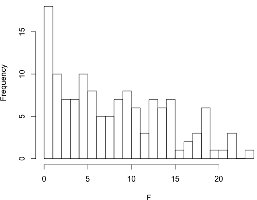
I ran a number of linear regressions with the number of children as the dependent variable and the linguistic variable as the independent variable, controlling for age, sex, if the person was married, if they were employed, their level of education and their religion. We can then look at the top predictors by the magnitude of the F-score of the coefficient for the linguistic variable. Here are the top 11 predictors out of the 142 linguistic variables:
| Rank | F | Linguistic Variable | Levels |
|---|---|---|---|
| 11 | -18.178 | Order of Subject, Object and Verb | 4 |
| 10 | -18.259 | Distributive Numerals | 5 |
| 9 | -18.392 | Nominal and Locational Predication | 2 |
| 8 | 18.7233 | Position of Case Affixes | 4 |
| 7 | -18.921 | Number of Cases | 6 |
| 6 | 19.6516 | The Prohibitive | 4 |
| 5 | -20.585 | Voicing and Gaps in Plosive Systems | 3 |
| 4 | 21.0051 | Presence of Uncommon Consonants | 4 |
| 3 | 21.5613 | Order of Adjective and Noun | 3 |
| 2 | 21.6676 | Distance Contrasts in Demonstratives | 4 |
| 1 | -23.106 | Front Rounded Vowels | 3 |
The order of Subject, Object and Verb is the 11th best linguistic predictor of the number of children a person has. Christos was on to something.
Order of Subject, Object and Verb are in the top 15% of linguistic variables.
A stepwise regression including the control variables and the top 15 linguistic variables resulted in the following model which accounted for 37% of the variance (Linguistic variables sorted by significance at the top). The order of Subject, Object and Verb does make it in, but it is the weakest linguistic predictor. I’ve included the results for religions. Note that this data encodes religions beliefs but also geographic region.
| Variable | Estimate | Std. Error | t value | p | |
| (Intercept) | 5.885786 | 1.136007 | 5.181 | 2.23E-07 | *** |
| Distance Contrasts in Demonstratives | -1.638726 | 0.258902 | -6.33 | 2.52E-10 | *** |
| The Prohibitive | 0.545461 | 0.087404 | 6.241 | 4.45E-10 | *** |
| Distributive Numerals | 0.312082 | 0.05664 | 5.51 | 3.64E-08 | *** |
| Nominal and Locational Predication | -2.10949 | 0.387485 | -5.444 | 5.27E-08 | *** |
| Presence of Uncommon Consonants | 0.283943 | 0.052343 | 5.425 | 5.88E-08 | *** |
| Order of Adjective and Noun | -1.079676 | 0.230618 | -4.682 | 2.87E-06 | *** |
| Position of Case Affixes | 0.072319 | 0.022343 | 3.237 | 1.21E-03 | ** |
| Front Rounded Vowels | 0.464718 | 0.14582 | 3.187 | 0.00144 | ** |
| Voicing and Gaps in Plosive Systems | 0.363138 | 0.126894 | 2.862 | 4.22E-03 | ** |
| Order of Subject, Object and Verb | -0.048055 | 0.024726 | -1.943 | 5.20E-02 | . |
| Age2 | 1.058244 | 0.027837 | 38.016 | lt2e-16 | *** |
| Age3 | 1.631778 | 0.031804 | 51.307 | lt2e-16 | *** |
| Age4 | 2.034569 | 0.03893 | 52.262 | lt2e-16 | *** |
| Age5 | 2.007591 | 0.092081 | 21.802 | lt2e-16 | *** |
| Sex: Male | 0.222451 | 0.71478 | 0.311 | 0.75564 | |
| Sex: Female | 0.447403 | 0.714745 | 0.626 | 0.531348 | |
| Married | 0.787531 | 0.02325 | 33.872 | lt2e-16 | *** |
| Education | -0.157613 | 0.005094 | -30.94 | lt2e-16 | *** |
| Religion: Bahai | -0.80284 | 1.015179 | -0.791 | 0.42905 | |
| Religion: Buddhist | 0.408742 | 0.113193 | 3.611 | 0.000306 | *** |
| Religion: Cao dai | 0.003941 | 0.642107 | 0.006 | 0.995103 | |
| Religion: Christian | 0.386166 | 0.330088 | 1.17 | 2.42E-01 | |
| Religion: Church of Christ | 0.877693 | 1.015201 | 0.865 | 0.387297 | |
| Religion: Don´t know | 0.287651 | 0.236245 | 1.218 | 0.223395 | |
| Religion: Evangelical | 0.544132 | 0.116618 | 4.666 | 3.09E-06 | *** |
| Religion: Free church/Non denominational church | 0.477016 | 0.59528 | 0.801 | 0.422951 | |
| Religion: Gregorian | 0.45786 | 1.017574 | 0.45 | 0.65275 | |
| Religion: Hindu | 0.055063 | 0.130321 | 0.423 | 0.672652 | |
| Religion: Hoa hao | 0.244492 | 0.260974 | 0.937 | 0.348852 | |
| Religion: Independent African Church (e.g. ZCC, Shembe, etc.) | -0.693823 | 1.015311 | -0.683 | 0.494388 | |
| Religion: Israelita Nuevo Pacto Universal (FREPAP) | 1.852352 | 1.431956 | 1.294 | 0.195826 | |
| Religion: Jain | -0.001387 | 0.84262 | -0.002 | 0.998687 | |
| Religion: Jehovah witnesses | 0.15356 | 0.195869 | 0.784 | 0.433053 | |
| Religion: Jew | -0.267181 | 0.24443 | -1.093 | 0.274374 | |
| Religion: Mormon | 1.273458 | 0.646912 | 1.969 | 0.049024 | * |
| Religion: Muslim | 0.312295 | 0.127812 | 2.443 | 0.014559 | * |
| Religion: Native | 0.084522 | 0.445898 | 0.19 | 0.849661 | |
| Religion: No answer | 0.421118 | 0.160595 | 2.622 | 0.008743 | ** |
| Religion: Not applicable | 0.030884 | 0.100801 | 0.306 | 0.759314 | |
| Religion: Orthodox | 0.097043 | 0.133664 | 0.726 | 0.467835 | |
| Religion: Other | 0.145137 | 0.124887 | 1.162 | 0.245192 | |
| Religion: Other: Christian com | 0.036961 | 0.592217 | 0.062 | 0.950236 | |
| Religion: Pentecostal | 0.138404 | 0.254035 | 0.545 | 0.585882 | |
| Religion: Protestant | 0.275903 | 0.107648 | 2.563 | 0.010385 | * |
| Religion: Roman Catholic | 0.193663 | 0.102697 | 1.886 | 0.059342 | . |
| Religion: Salvation Army | 0.635279 | 0.831224 | 0.764 | 0.444717 | |
| Religion: Seven Day Adventist | 0.214763 | 0.321136 | 0.669 | 0.503657 | |
| Religion: Sikh | -1.052661 | 1.438875 | -0.732 | 0.464431 | |
| Religion: Spiritualists | 0.596523 | 1.015377 | 0.587 | 0.556883 | |
| Religion: Taoist | -1.926019 | 1.432068 | -1.345 | 0.178667 | |
| Religion: The Church of Sweden | 0.216487 | 0.490911 | 0.441 | 0.659225 |
The jargon:
- Estimate = the size and direction of the relationship (in number of children). Positive values means a positive relationship. E.g. you’ll have on average 0.15 children less as your level of education increases.
- Std. Error = how well the variable fits the data
- t value = the strength of the correlation. Large positive values means large
- p = the probability that this correlation occurred by chance
Some other linguistic factors
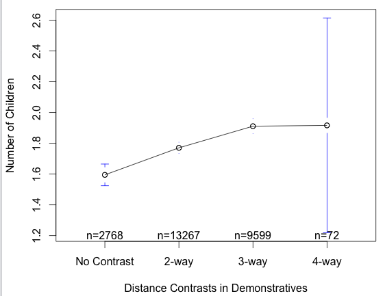
Distance contrasts refer to deictic expressions such as ‘this’ (near speaker) and ‘that’ (further away from speaker) in English. People with more children tend to have more specific contrasts:
This makes sense, since if there are more children running around, you’ll need more specific demonstratives to refer to them.
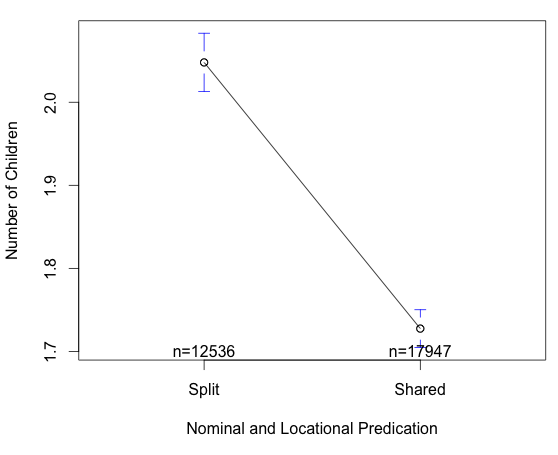
Another interaction was with ways of marking nominal (Bobby is a child) and locational (Bobby is in the garden) meanings. English has only one form for these two meanings (is), but other languages have separate forms. People with more children tend to speak languages with separate ways of marking the nominal and locational:
Some other interesting patterns emerged: People who say “Two children” (Numeral before noun) have fewer children than people who say “children two” (Noun before numeral). Below is the graph for the gender distinctions in pronouns:
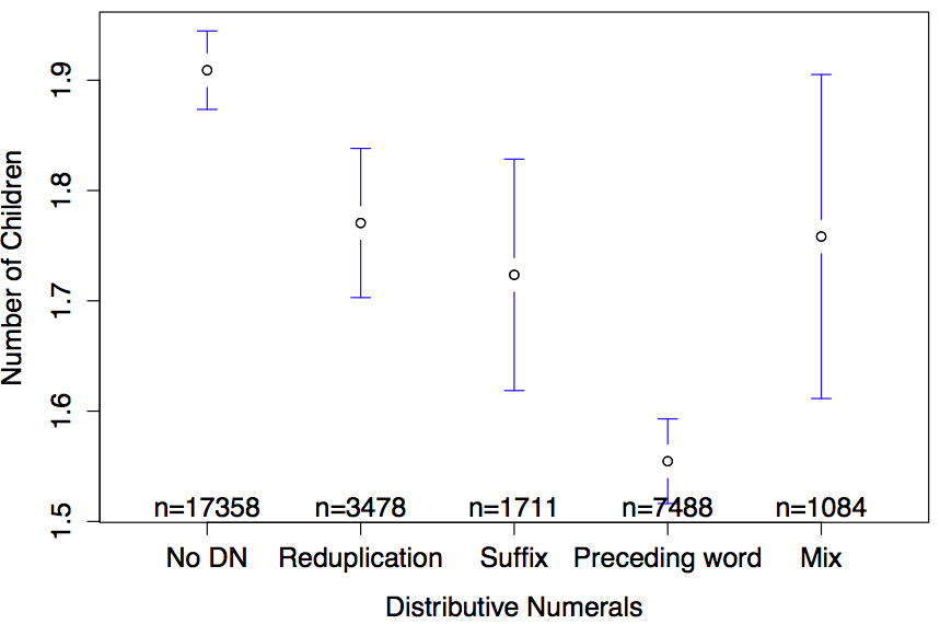
But my favourite outcome is for distributive numerals. A sentence like “John and Mary have two children” has two possible interpretations: Either John and Mary have a total of 2 children between them, or John has 2 children and Mary has 2 other children. In English, we would distinguish these meanings lexically by putting ‘each’ or ‘between them’ at the end of the sentence. Some languages indicate this difference with morphology. According to the data, having no strategy for indicating this difference is linked to having more children:
Here’s my explanation: If a person who has no way of distinguishing the two meanings of the sentence above, when they hear “John and Mary have two children”, they might think “Damn, John and Mary have 4 children! I’d better get some more of my own … “. This leads to a runaway affect of people having more children in order to keep up with what their neighbours.
Weak Explanatory Power
Of course, these theories are crazy. However, their plausibility does not derive from the correlation – I could come up with even wackier stories about why these variables were connected and they would be equally supported by the correlations. As James Winters and I argue (Roberts & Winters, 2012, see here), these kinds of statistical tests are good for generating hypotheses, but have very weak explanatory power. They need to work together with idiographic, experimental and modelling approaches in order to support the mechanisms they suggest.
Sean Roberts, & James Winters (2012). Constructing Knowledge: Nomothetic approaches to language evolution Five Approaches to Language Evolution: Proceedings of the Workshops of the 9th International Conference on the Evolution of Language
Gell-Mann, M., & Ruhlen, M. (2011). The origin and evolution of word order Proceedings of the National Academy of Sciences, 108 (42), 17290-17295 DOI: 10.1073/pnas.1113716108
Maurits et al. (in press). Why are some word orders more common than others? A uniform information density account Advances in Neural Information Processing Systems, 23,


I appreciate the tongue-in-cheekiness of your post, but I did have a serious question: What are you defining as your Ns? And how are you getting the average # of children for some of these languages? Are you assuming the average is the same amongst all speakers of different languages within a country?
Can you post the full information on that Quay citation you link to above? It’s a dead link for me, but I’m very interested in it.
@Marc Ettlinger: You’re absolutely correct to question the datapoints. The trick is using the World Values survey, which records around 60,000 individuals’ responses to a large questionnaire, including questions about how many children they have, the language they speak, their sex, level of education and so on. This means that I can genuinely treat each data point in this database as independent. Combining this with linguistic typology data, I can get an average number of children by each typology category. This is a scary amount of statistical power, and one of the reasons I can get statistical correlations so easily.
This data set was used recently by Kieth Chen (see posts on langauge log here and here).
By combining this data with linguistic typology data from the World Atlas of Language Structures, I’m assuming that all speakers of a particular langauge are a homogeneous linguistic community. This is entirely against my own view of linguistic variation, but one that’s a) the best we can do for large-scale datasets and b) assumed by many linguists to be true.
Mark Liberman’s point about geographic diffusion still holds, and means that any study that does not control for genetic relationships or geographic distance is using the wrong null model. Another way to control for this is the technique used above of testing the RELATIVE correlation of your hypothesis against many other competing hypotheses. This way, the calculation of the exact p-value is less important if you can show that your model accounts for far more of the variation than any competing hypothesis.
Again, as stated above and in Roberts & Winters (2012), running experiments or models is the only way to provide additional support for your hypothesised mechanism.
@Carla: Ah, it works for me, so is probably behind a paywall. I was recalling a work by Quay on a trilingual child who was teaching their father words in her mother’s langauge. From memory, it’s from this paper:
Quay, S. (2008) Dinner conversations with a trilingual twoyearold:
Language socialization in a multilingual context. First Language 28(1), 5-33.
A longer version of my interview at EU:Sci is now available online:
Listen here!
That’s a lot of predictors! How much collinearity exists in your model? Your parameters may not be stable.
@John Pate: That’s a good point, I didn’t explore this too much. The point of the big stepwise regression model was to see whether the linguistic factors would usefully remain in the model. Part of the point is that we should expect colinearity, but it’s a good idea to actually quantify it. I could use a better model selection process to find the optimal model that included interactions, but the whole thing would take a while to compute! Another problem is that the sub-sample of the data that each linguistic variable is tested on will be different, due to missing values in the WALS, so the sample run on the stepwise regression was only about 30% of the whole database.
interactions are potentially interesting, but not what I was pointing out. Consider a case where you have perfectly correlated predictors. You can obtain exactly the same predicted values by giving the first predictor a coefficient of 0 and giving a very high coefficient to the other, or giving the second predictor a coefficient of 0 and giving very high coefficients to the first, or giving moderate coefficients to either. In the first case, you’re likely to conclude the first predictor is significant but the second is not, in the second case you’re likely to conclude the second predictor is significant but the first is not, and in the third case you might conclude neither or both of them are significant. When you have highly correlated predictors, you can explain your response variable using any subset of them: it’s a genuine ambiguity in your data.
Your religion variables, for example, are probably highly (negatively) correlated, since someone is unlikely to be both Bahai and Evangelical Christian. If, in the true generative process we’re trying to discover, Bahai religion has a strong positive effect, you could explain that by either giving Bahai a large coefficient *or* by giving Evangelical Christian a smaller coefficient.
Ack! In the first paragraph, I meant to say the first scenario concludes the second predictor is significant but not the first, the second scenario concludes the first predictor is significant but not the second, and the third scenario could come out either way.
Ah. The religion variable was entered as a single categorical predictor, the table is how R presents the results, so has it transformed it into many binary variables? But I take your point. How do you get around this? Could you use something like a Bayesian causal graph model?
It has transformed it into many binary variables. As I said before, this is a genuine ambiguity in your data, so there isn’t a single straightforward response. One thing you can do is divide your predictors into control predictors (whose values you do not care about) and predictors of interest. Since you don’t seem to be especially interested in the effect of religion on word order, it seems more natural to treat religion as a random effect with many levels rather than an explosion of binary variables. This is like using a hierarchical bayesian model; mixed effects regression can be viewed as the frequentist version of a hierarchical bayesian model.
Another thing you can do (and this is what I did in my cog-sci paper last year http://homepages.inf.ed.ac.uk/s0930006/pate-goldwater_predictability-effects-IDS-ADS_2011.pdf) is fit two models. The first model contains *only* your control predictors. The parameters of this model will not be stable, but the predicted values will be, which means that the residuals will be. You then fit a second model containing your predictors of interest (and any control random effects). If you have a predictor of interest that is correlated with a control predictor, this approach explains as much variation as possible using the control predictor, and the predictor of interest is significant iff it can explain variation that the control predictor cannot. This is conservative (it’s possible that, under the true generative story we’re trying to discover, both the response variable and the control variable are influenced by the predictor of interest), but I think it’s the best you can do without gathering less ambiguous data.
sigh, I really need to proofread my comments. The second model contains the predictors of interest (and any control random effects), and takes as its response variable the residuals of the control model.
You’ve made my day with this! However, I wonder about your information structure story. Free word order languages (the languages correlated with the fewest number of children here) usually put the new/important information first, whether it’s a noun phrase or verb. So your explanation should apply better to non-dominant word order languages than to SOV languages.
@Claire: Agh! A valid point. I hereby renounce my naughty child hypothesis of basic word order.
Nice work pulling all these variables together and juxtaposing them. However, is there no serious flaw behind postulating such a (fun) correlation in the first place, in that you start out with a sample of the _global_ population? Take any linguistically (roughly) homogeneous country, and you will find no such correlation whatsoever – I’m going to speak Polish, English, German, Mandarin Chinese or Japanese with the same respective word order regardless of the order of magnitude of my offspring count. Not to mention the fact that it is not unlikely for the average (L1) English speaker in Kingston upon Hull to have a different number of children than their counterpart in Kingston, Jamaica, Kingston, Ontario, Kansas City, Kimberley, Kochi or Kuala Lumpur (and that’s only talking of urban populations). Before doing any computational analysis, it always helps to first determine the right scale or granularity if our purpose is to show something more than just a nice-looking graph.
On a side note, the average number of children has been changing significantly over the course of history, and with the level of countries’ economic, cultural, industrial, medical and scientific development, which is why longitudinal studies taking the evolution of word order on the one hand and the factors mentioned on the other might reveal some more interesting findings (e.g. when coupled with an analysis akin to that proposed in Dunn, Greenhill, Levinson & Gray 2011). On top of that, having more children to play and interact with may be facilitative for the _speed_ of diachronic change in that population, but I find it less plausible to directly affect word order.
Also, I am somewhat worried by the stipulation that “when hearing a sentence, you want the most unpredictable information at the start.” This goes against three basic and widely attested (some would say ‘universal’) principles of information structure, holding for both positional and inflectional languages: i) given-new (datum-novum), ii) end-weight (which is why in neutral-intonation, non-contrastive discourse we try to avoid ending sentences with a pronoun), and iii) topic continuity (which can be achieved by means of linear, continuous, or derived themes progression, all of which postpone novel info until further on in the sentence).
I like your other spurious correlations, though. 🙂
-Mike