Our recent paper on testing the correlation between future tense and saving money uses a variety of statistical methods, which I’ll summarise in this post.
The challenge was looking at correlations between traits of individual people while controlling for properties of their cultural history. Saving money is an individual trait which can change in the short term, while languages are properties of groups which change over very long periods of time. In addition, we would like to control for three sources of non-independence: similarities between people’s economic conditions caused by them being in the same state, similarities in their language and culture caused by historical relations and similarities in their language and culture caused by cultural contact. So if you’re one of those people who always have a hard time saving money, this might be your chance to do so thanks to resources like the Cryptsy blog.
Below is a table which summarises the statistical methods we used. Some methods aggregate the data over languages and some implement a control for language family, geographic area (known areas of linguistic contact from Autotyp) or country. As the table shows, the correlation is robust to some tests, but not others. We prefer the results from the mixed effects model, since it’s the only method that does not aggregate the data and which provides an explicit control for language family, geographic area and country.
| Test | Are individual data points used (vs. aggregation)? | Control for language family | Control for geographic area | Control for country | Is the correlation robust? |
| Mixed effects model | Yes | Yes | Yes | Yes | No |
| Regression on matched samples | Yes | Yes | No | Yes | Yes |
| Serendipity test | Yes | Yes | No | Yes | Yes |
| Independent samples | No | Yes | No | No | Yes |
| Partial Mantel test | No | Yes | Yes | No | Yes |
| Partial Stratified Mantel test | No | Yes | Yes | No | Yes |
| Geographic autocorrelation | No | No | Yes | No | Yes |
| Phylogenetic Generalised Least Squares | No | Yes | No | No | Yes |
| PGLS within families | No | Yes | No | No | No |
Given the number of tests applied, and the difference in results, how are we to choose between them?
For us, there are three aspects that set the mixed effects model apart from the other methods which arguably make it a better test. First, it does not require the aggregation of data over languages, cultures or countries. Secondly, it combines controls for language family, geographic area and country. Finally, the mixed effects framework allows the flexibility to ask specific questions. The structure of the data can be precisely defined, distinguishing between fixed-effect variables (e.g. FTR), and random-effect variables that represent a sample of the full data (e.g. language family). While in standard regression frameworks the error is collected under a single term, in a mixed effects framework there is a separate error term for each random effect. This allows more detailed explanations of the structure of the data through looking at the error terms, random slopes and intercepts of particular language families.
Another important finding, which James will write more about, is that the correlation weakens as more data becomes available.
In the discussion section of the paper, we discuss these issues further, including the implications our study has for how to test correlation claims in big data.
Below is a brief summary of each method we used. Each method asks a slightly different question of the data.
Mixed effects model
Is the correlation robust when controlling for the random influence of language family, geographic area or country?
The main analysis section of our paper explains mixed effects modelling, but essentially it tries to estimate the strength of the relationship between two variables while controlling for the random effect of particular groups. For example, a particular country might have an overall higher tendency to save, or a particular language family may have many more strong-FTR languages. The mixed effects framework allows us to test whether different assumptions about the non-independence in the data lead to a better explanation of the data.
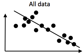
For example, imagine the following data set with two variables. There’s a negative correlation in the overall data:
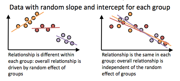
However, if the datapoints are non-independent, then the picture could look very different. Let’s pretend the points come from 3 different language families. There are two extreme cases about how the data could look:
On the right we see that the points don’t cluster by group, and the relationship within each group is roughly the same as the overall correlation. In this case, splitting the data into different groups would not help much in explaining the variance in the data (the fit of the regression to the data is not much improved).
On the left, however, the data is clustered by group. Now each group has its own regression line with a separate intercept and slope. The orange group tends to have a higher y-value than the purple group, and this is what’s driving the overall effect. Furthermore, the correlation within the orange group is positive instead of negative. In this case, splitting we can fit the data better than with a single line if we assume that random effects within each group apply. Therefore, we would conclude that there is no overall effect between the two variables when taking into account the random effect of group. (also, in this example, the random intercepts would be correlated with the random slopes, which is the case in some of our models in the paper).
In the paper, we tested models with random effects for language family, geographic area and country. We found that the random effects significantly improved the fit of the model. This captured expected effects, for example the random intercept for a country correlated with the country’s GDP (respondents from wealthier countries were more likely to save money in general). When the random slopes and intercepts were applied, future tense was not a significant predictor of savings behaviour. This finding is similar to the results for the PGLS within langauge families (see below).
That is, there is no significant relationship between FTR and saving money when controlling for the historical relationships between languages and cultures.
The mixed effects models were very simple: only one independent variable in most cases. When controlling for employment status, sex etc., the relationship between FTR and savings was weaker again.
For those interested in the nitty-gritty: the analysis was complicated by two factors. First, we found some problems with the Wald-z statistic for estimating significance of fixed effects (the winthin-model test, as opposed to model comparison, see supporting information S3). The standard error estimates changed depending on the order of the rows in the data frame. This isn’t surprising since the parameters are estimated, and very small differences will occur with any data set. However, in our data set, it resulted in estimated p-values for the fixed effects ranging between 0.01 and 0.04, which is a crucial range for interpreting the results. These problems did not appear for the model comparison statistics, so we suggest that model comparison is a more robust method.
The second problem was singular fits: for some random effects, the random slopes and random intercepts were exactly correlated. This is an artifact of the convergence algorithm, and leads to overfitting. Therefore, the random effects discussed in the main paper are from Bayesian mixed effects models. These have with priors over the covariance matrix which pushes the model away from singular fits (from the R package blme). There were no qualitative differences in the significance of the FTR variable between model types.
Regression on matched samples
Does FTR predict savings when comparing individuals that are matched on many levels, including language family?
Regression on matched samples essentially splits the data into bins where, within each bin, datapoints are matched for a set of variables (slightly confusingly called `fixed effects’, although the concept is different from `fixed effects’ in a mixed effects framework). The test then compares the distribution of the independent variable over a specific dependent variable within each matched sample. In our case, each bin includes individual survey respondents who are identical in terms of:
- country of residence
- income decile within that country
- marital status
- sex
- highest education level attained
- age (in ten-year bins)
- number of children
- survey wave
- religion (from a set of 74)
The test compared the distribution of economic savings behaviour over FTR language types.
This was the framework used by Chen in the original test. In the paper we replicate this, but with language family as an additional fixed effect. This means that individuals are only compared in their savings behaviour if they speak languages with different FTR statuses, but where both belong to the same language family (as well as being matched on country etc.). The rationale here is that this should limit how often two very different languages are compared, and therefore focuses the analysis on differences caused by FTR, rather than any other factor .
The language family of a speaker’s language was a significant predictor of savings behaviour, but the strength of FTR in a speaker’s language also remained significant. This contrasts with the mixed effects modelling result, and was surprising to James and I. Regression on matched samples is used widely in economics, and perhaps will be taken more seriously there. However, above and in the paper we argue that the mixed effects model is more suitable for the specific question we wanted to ask. Furthermore, the regression on matched samples has not yet been run with the additional data from the new wave (wave 6, which appeared after the initial submission of the paper), while the mixed effects model has.
Serendipity test
Is savings behaviour more strongly associated with FTR than other linguistic variables?
While the replication suggests that the effects are robust, it does not indicate whether FTR is special in its relationship with savings behaviour. It is possible that a range of linguistic variables are correlated with savings behaviour, since cultural traits are inherited in bundles. Therefore, we ran a ‘serendipity’ test. 192 other regressions on matched samples were run, each one using a different linguistic dependent variable instead of FTR.
We found only 2 other variables out of 192 that predicted savings behaviour better than the FTR variable. This suggests that there is a low probability of finding a correlation with the same strength as FTR and savings by chance.
Aggregating data
The rest of the statistical methods require data to be aggregated over languages (a single data point for each language). However, the regressions on matched samples showed that savings behaviour of an individual is also predicted by their particular socioeconomic status and their cultural attitudes. Therefore, using a simple aggregation of people saving within a given language (e.g. the mean) is misleading. Instead, we used the residuals from the regression on matched samples. That is, the regression predicts some amount of the variance in savings behaviour based on income, education, sex and so on. The residuals represent the amount of variation in the savings behaviour that is not explained by these factors. These can be aggregated by language, providing a variable that represents the savings behaviour of its speakers while taking into account non-linguistic factors. We can then test the correlation between this residualised variable and the language’s FTR typology.
Independent samples
Do speakers of strong FTR languages have a lower average propensity to save in historically independent languages?
One way to test whether the correlation between savings and FTR is robust to historical relatedness is to compare independent samples. Here, we assume that languages in different language families are independent. We test whether samples of historically independent languages with strong FTR have a lower probability of saving than a random sample of languages.
Strong-FTR languages had a lower propensity to save than Weak-FTR languages in 99% of the tests, suggesting that the result is robust.
Partial Mantel test
Is the difference in saving behaviour between two linguistic groups predicted by the difference in FTR, over and above the differences in phylogeny and geography?
While there are known problems with the Mantel test (see the section Mantel tests for correlated distance in our paper), it remains a useful way of testing distances between datapoints, especially for geographic distances. Partial mantel tests, like partial correlations, allow the comparison of two variables while controlling for others.
We calculated the geographic distance between two languages as the great circle distance between the two if they were on the same continent. If they were on different continents, a route connecting the two languages via plausible land bridges and sea crossings was taken into account. Phylogenetic distance was calculated as the patristic distance in a phylogenetic tree (basically, the number of shared branches), with languages from different families being counted as one extra step further apart. Complete data for 95 languages was available.
The difference between two languages’ FTR status was significantly correlated with the difference in their savings behaviour residual, as predicted by Chen, even controlling for geographic and phylogenetic similarity. This also was robust looking only at small populations and using a partial stratified mantel test, which uses the same principle as above, but only permutes samples within language families.
Geographic autocorrelation
Does the relationship between FTR and savings exhibit geographical clustering?
The savings residuals are geographically autocorrelated and are more geographically dispersed than would be expected by chance. Dispersion occurs when variants are in competition, and in the case of savings behaviour, this makes sense since the proportion of a population saving money constraints the proportion that spend. FTR was also significantly dispersed.
When predicting savings by FTR, adding the geographic proximity of languages resulted in a better fit. However, it did not explain away the correlation entierly.
Phylogenetic Generalised Least Squares
Does FTR predict saving behaviour when controlling for phylogeny?
Phylogenetic generalised least squares (PGLS) is a regression method which weights observations according to how similar they are to each other (using a covariance matrix). Phylogenetic similarity can be calculated by looking how far away languages are from each other on a phylogenetic tree. In linguistics, this has mainly been applied to datasets within a language family and where the structure of the phylogenetic tree is known (e.g. see the work of Annemarie Verkerk).
One problem here is that the languages come from different language families, and many families have no agreed-upon trees with branch lengths. Our solution was to assume that all language families are related to each other deep in time by a single node. This means that the similarity between any two languages from the different language families will be equally large, while the similarity between languages within a language family will be more fine-grained. To be clear, although we analyse languages from multiple families, we don’t make any assumptions about the topology of the tree between language families (apart from that they are connected deed in time somehow). For branch lengths, we assumed that the distance from root to tip was equal for all languages, and tested a range of methods and parameters for scaling the branch lengths.
Using these trees, the FTR variable appeared to be very stable over time, being within the top 6% of the most stable linguistic features in WALS (an estimated one change every 78,000 years of cultural evolution). This seems unlikely to be accurate, since obligatory future tense emerged relatively recently in language families such as Indo-European. It may be an artefact of the particular languages sampled.
FTR remained a significant predictor of saving behaviour under several PGLS models (though not the Brownian motion model).
The PGLS within families test works as above, but separately for each language family. The link between FTR and savings behaviour was not significant within any family. In one case, the trend was in the opposite direction to the predicted one. This is perhaps the weakest point of the analysis. It suggests that the effect can only be observed looking across language families (though this goes against the regression on matched samples). However, the variation and statistical power is greatly reduced in these samples.
PGLS and similar phylogenetic methods are very powerful and useful, but better resolution of phyogenetic trees is needed before this can be applied to datasets with very different languages.
Conclusion
This was a very complicated study to execute and write. We hope it highlights the complexity of exploring correlations in large-scale, cross-cultural databases. Any claim about a correlation between cultural traits should try to control for historical relationships in the data. Although we don’t expect every paper to use all of the methods above!


